Ballast-tank sloshing — the 2D CFD study
From analytical natural periods to CFD-benchmarked resonance: a partially filled tank has a gravity-driven sloshing mode; tune it near a vessel's roll period and it acts as a passive tuned-liquid (anti-roll) damper. This page showcases the 2D VOF CFD that pins the analytical master curve to measured data and shows how forced roll excites the resonance.
VERIFIED · real OpenFOAM v2312
1 · Natural period — CFD vs analytical (without forced roll)
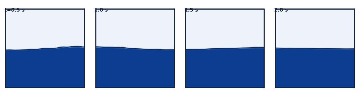
A free-decay run rings down a small first-mode perturbation in a static rectangular tank; the FFT natural frequency, non-dimensionalised as Ω₁ = ω₁√(L/g), is compared to the analytical linear-potential value √(π·tanh(πh/L)). Four fills bracket the curve.
— analytical ◯ measured CFD (free-decay, no forced roll)
| Fill h/L | Ω₁ measured (CFD) | Ω₁ analytical | Error |
|---|---|---|---|
| 15% | 1.1779 | 1.1746 | 0.28% |
| 30% | 1.5164 | 1.5210 | 0.30% |
| 50% | 1.6974 | 1.6974 | 0.00% |
| 70% | 1.7508 | 1.7508 | 0.00% |
Result. The 2D VOF pipeline reproduces the analytical first-mode frequency to within 0.30% across the fill range — the measured points sit on the rectangular master curve. See the CFD-vs-literature chart (which shape was validated) in the interactive explorer.
Grid & timestep convergence — is the ≤0.30% earned?
The literature (and our own adversarial review) is clear that a sub-percent match must be earned by a convergence study, not asserted. This refines the exact case with the known ~0.30% error (L=1 m tank, h/L = 0.30 — which lands on a cell face at every mesh, so the analytical target is identical) across five grids and three timesteps.
Free-decay frequency error vs mesh — it falls only slowly toward a ~0.29% floor: the residual is physical (finite-amplitude), not mesh.
| Mesh | Cells | Freq (Hz) | |error| | Runtime (s) | Predicted (s) |
|---|---|---|---|---|---|
| 40×40 | 1,600 | 0.75558 | 0.326% | 149 | 117 |
| 60×60 | 3,600 | 0.75565 | 0.317% | 241 | 264 |
| 80×80 | 6,400 | 0.75570 | 0.310% | 342 | 470 |
| 120×120 | 14,400 | 0.75576 | 0.302% | 684 | 1,058 |
| 160×160 | 25,600 | 0.75581 | 0.296% | 1,208 | 1,881 |
The last two columns check the run-time estimator: its rate is calibrated at ~16-wide contention, so it reads as an upper bound here — this batch ran 7-wide and tapering, so actual came in below predicted, exactly as the contention model says (fewer concurrent → faster per case).
Timestep sweep (fixed 80×80 mesh)
| Δt (s) | Timesteps | Freq (Hz) | |error| |
|---|---|---|---|
| 0.004 | 3,000 | 0.75570 | 0.310% |
| 0.002 | 6,000 | 0.75570 | 0.310% |
| 0.001 | 12,000 | 0.75572 | 0.308% |
Richardson extrapolation (ratio-2 triple). Observed order of accuracy p = 0.191, grid-converged frequency 0.756556 Hz vs analytical 0.758054 Hz, fine-grid GCI = 0.1239%. The extrapolated value stays ~0.2% below the linear-analytical target, and p is far below the formal ~2 — so the study is not in the asymptotic regime and the GCI is indicative only (a non-mesh term dominates the error).
Verdict. Numerically sound: the frequency is grid- and timestep-converged — mesh error falls monotonically to a ~0.29% plateau (only the finest 25,600-cell mesh reaches ≤0.30%) and the timestep sweep is flat over a 4× refinement. But the residual is predominantly PHYSICAL, not discretization: Richardson extrapolation gives 0.7566 Hz, still ~0.20% below the linear-analytical 0.758 Hz — an irreducible finite-amplitude offset (0.02 m perturbation) from the linear tanh dispersion. The low observed order (p ≈ 0.19, far below the formal ~2) confirms a non-mesh term dominates the error budget, so the GCI (0.12%) is indicative only. Bottom line: the ~0.3% agreement is a finite-amplitude modeling difference, not numerical error that vanishes with refinement.
2 · Forced-roll resonance — with vs without
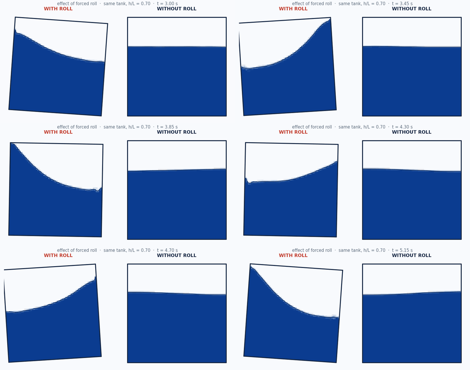
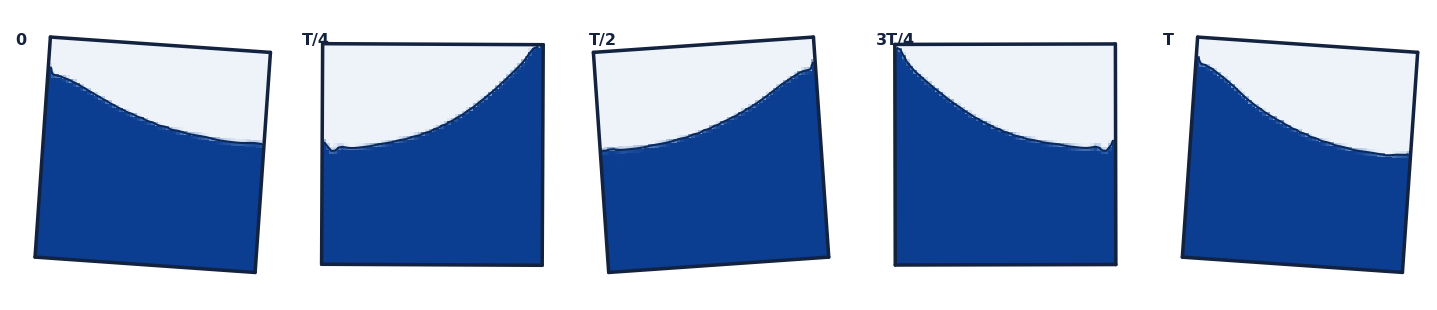
Without forced roll, the free-decay run gives the intrinsic natural period. With forced roll, driving the tank (4.0° roll) at a range of roll periods and measuring the steady wall run-up traces a resonance curve that peaks at that same natural period — roll excites the mode the free-decay rings down. The dashed grey curve is the linear damped-oscillator amplification (Faltinsen & Timokha 2009; Abramson 1966).
● fill h/L = 0.3 ● fill h/L = 0.5 ● fill h/L = 0.7 – – damped-oscillator model (ζ = 0.170)
| Fill h/L | Natural T₁ analytical (s) | Natural T₁ free-decay CFD (s) | Resonant T forced CFD (s) | resonant / natural |
|---|---|---|---|---|
| 30% | 1.251 | 1.247 | 1.251 | 1.00 |
| 50% | 1.121 | 1.117 | 1.121 | 1.00 |
| 70% | 1.087 | 1.089 | 1.087 | 1.00 |
Confidence. At every fill the forced-roll resonant period lands on the natural period (ratio ≈ 1.00). Roll excitation and free decay agree on the same mode — the methodology is self-consistent.
3 · Roll-amplitude backbone — amplitude-dependent detuning
At 4° roll the resonant peak sits on the linear T₁ (section 2). Nonlinear theory predicts this only holds at small amplitude: the fundamental sloshing mode is a soft spring whose resonant frequency drifts with amplitude. This sweep drives each fill at 2–8° over a frequency grid and locates resonance by the quadrature (damping) coefficient peak — the phase-based locator (Bäuerlein & Avila 2021); the wall run-up saturates near resonance and is not a reliable locator, so it is reported separately.
● h/L = 0.3 (near / below critical depth) ● h/L = 0.7 (above critical depth)
| Fill h/L | Roll amp | Resonant T/T₁ | Freq detuning | Peak run-up (m) |
|---|---|---|---|---|
| 30% | 2° | 1.009 | -0.92% | 0.255 |
| 30% | 4° | 1.054 | -5.10% | 0.422 |
| 30% | 6° | 1.094 | -8.60% | 0.419 |
| 30% | 8° | 1.121 | -10.81% | 0.432 |
| 70% | 2° | 1.046 | -4.38% | 0.339 |
| 70% | 4° | 1.088 | -8.06% | 0.390 |
| 70% | 6° | 1.122 | -10.89% | 0.404 |
| 70% | 8° | 1.153 | -13.25% | 0.409 |
Result. Both fills show soft-spring detuning: the resonant frequency drops monotonically as roll amplitude grows, reaching ~11–13% below f₁ at 8° (h/L = 0.30: −0.9% → −10.8%; h/L = 0.70: −4.4% → −13.2%). The h/L = 0.70 case (above the h/L ≈ 0.34 critical depth) is the clear soft spring; h/L = 0.30 sits right at the critical depth and also detunes downward under strong shallow-water nonlinearity rather than showing the clean hardening small-amplitude theory would predict. So “resonance at T₁” is the small-amplitude limit only — at operational roll angles the tank detunes, and anti-roll tuning must use the amplitude-annotated value. (The base grid is Δr = 0.05; the h/L = 0.70 grid was extended to r = 1.25 at 6–8° so the strongly-detuned peak is now bracketed interior — the 8° peak was previously clamped at the r = 1.15 edge, i.e. a lower bound; the de-clamped value is −13.2%. Values reduced with the corrected sub-grid vertex interpolation introduced with the shallow-fill sweep — the originally published detunings placed each peak correctly only to the Δr = 0.05 grid.)
External validation — Delorme / SPHERIC Test 10 (shallow fill, impact pressure)
The one recognised external benchmark with published experimental data (not our own analytical): the SPHERIC
Test 10 lateral-impact case (Delorme et al. 2009; benchmark values Botia-Vera et al. 2010). A shallow-filled
tank (L=0.9 m, h=0.093 m ≈ 18% fill)
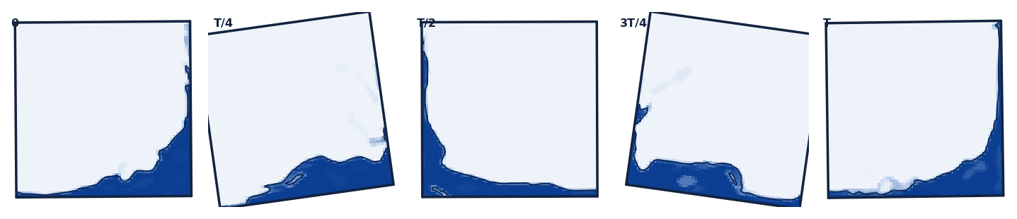
in 4.0° forced roll at T=1.6298 s (0.85·T₀) throws an
overturning wave that slams the side wall at the still-water line; the first-impact pressure at Sensor 1
(y=0.093 m) is the validated quantity. A moving-wall patchProbes tap tracks the
rotating wall.
| Quantity | Value | Note |
|---|---|---|
| CFD first-impact peak (Sensor 1) | 4,688 Pa | single 2D interFoam realisation |
| Experiment, first-peak (water, 1X) | 3,710 ± 732 Pa | mean ± SD, 100 runs (CoV ~19.7%) |
| Experimental 2σ band | 2,246–5,174 Pa | CFD / mean = 1.264 |
Within the experimental scatter. The CFD peak sits at 1.264× the experimental mean (upper part of the 2σ band) — consistent with the documented tendency of violent-impact CFD/SPH to over-predict pressure maxima. A single deterministic 2D CFD run is one draw from a strongly stochastic impact distribution (experimental CoV ~20%), so agreement is judged as landing within the experimental scatter, not as an exact number; 2D also omits the experiment's out-of-plane-thickness dependence and air entrapment. This validates the forced-roll VOF impact path against measured data at shallow fill.
Sources: Botia-Vera, Souto-Iglesias, Bulian & Lobovsky (2010), Table II (100 runs); Delorme et al. (2009), Ocean Eng. 36(2).
Shallow-fill bore regime — amplitude sweep at h/L = 0.15
The fills above sit at or above the h/L ≈ 0.34 critical depth. Real ballast operation also passes through shallow fills, where the response is set by travelling bores / hydraulic jumps and low-order (tanh-dispersion) theory degrades — the regime where anti-roll tuning must come from CFD. This refined sweep drives h/L = 0.15 (h = 0.135 m) at 1–8° roll over a fine Δr = 0.025 frequency grid with 16-cycle records (38 cases; the 2° case is refined to a Δr = 0.0125 half-step for a grid-convergence check). The free-decay benchmark (section 1) anchors the small-amplitude natural frequency at this fill to within 0.28% of linear theory; the sweep measures how fast that anchor degrades as amplitude grows. Resonance is located by the quadrature (damping) coefficient peak. Bore onset is tracked by two wall-probe indicators: run-up / depth (the shallow-water nonlinearity parameter) and crest/trough asymmetry (bores throw a sharp high crest over a drawn-down trough; a linear standing wave is symmetric).
● roll 1° ● roll 2° ● roll 4° ● roll 6° ● roll 8° — each curve normalised to its own peak; the peak location is the resonance.
| Roll amp | Resonant T/T₁ | Freq detuning | Peak run-up / h | Crest/trough asymmetry |
|---|---|---|---|---|
| 1° | 0.930 | +7.49% | 1.633 | 4.385 |
| 2° | 0.935 | +6.98% | 1.890 | 4.209 |
| 4° | 0.944 | +5.96% | 2.356 | 3.685 |
| 6° | 0.973 | +2.77% | 2.554 | 4.119 |
| 8° | 0.988 (≈ within resolution) | +1.23% | 3.090 | 4.955 |
Run-up / h and asymmetry are each amplitude's maximum across the ratio grid; they occur near (not exactly at) the resonant ratio. Off resonance both indicators fall sharply — toward the edges of the swept band the run-up drops well below its resonant value and the asymmetry falls toward 1. “≈ within resolution” flags an amplitude whose quadrature peak is flat enough that the detuning is within grid/method resolution of the linear anchor (sign-consistent only).
● h/L = 0.3 (near / below critical depth) ● h/L = 0.7 (above critical depth) ● h/L = 0.15 (shallow-water / bore regime)
Result. Below the h/L ≈ 0.34 critical depth the shallow fill detunes the opposite way to the deeper fills: a hardening response with the resonant frequency above linear f₁ at every amplitude (the sign flip nonlinear theory predicts below critical depth; Faltinsen & Timokha 2009). This is now grid-resolved, not a sub-grid artifact: on the refined Δr = 0.025 grid the quadrature-peak node itself walks with amplitude (0.925@1° → 0.9375@2° → 0.95@4° → 0.975@6° → 1.0@8°). A half-step Δr = 0.0125 convergence check at 2° holds the peak at r ≈ 0.935, so the sub-grid vertex is confirmed, not manufacturing the trend. The flip is between h/L = 0.15 and the 0.30/0.70 fills; our h/L = 0.30 case, nominally just below critical, already softens, so the practical boundary sits below 0.30 rather than exactly at 0.34. The hardening weakens monotonically as roll grows — from ~+7% at 1° to ~+1% at 8° (within grid/method resolution of the anchor — sign-consistent only). That is not a clean hardening backbone (which would bend away from f₁ as amplitude grows); it is the signature of bore dissipation — the travelling bore breaks harder at higher amplitude, broadening the peak and pulling the effective resonance back toward T₁. Correction. An earlier 8-cycle coarse-grid (Δr = 0.05) sweep placed every amplitude's peak at r = 0.95 and reported the hardening as indicative. The refined 16-cycle Δr = 0.025 sweep supersedes it: the low amplitudes are confirmed (within ~±0.4 pct-pt), but the high amplitudes were overstated by ~2 pct-pt (6°: +4.8% → +2.8%; 8°: +2.9% → +1.2%) — the short records had not settled near resonance. The 1° anchor (+7.5%, the strongest swept) shows the hardening does not reverse above 1°; reconciliation with the near-zero free-decay anchor (natural frequency within 0.28% of linear at ≈0 amplitude) therefore happens only in the un-swept sub-1° limit — and note free decay (unforced transient frequency) and forced phase-resonance coincide only in the linear limit, so part of that gap is definitional. What is not in doubt is the violence: near resonance even 2° roll is a bore-like wave, run-up 1.6× the still depth (rising to ~3× at 8°) and crest/trough asymmetry ~4–5 (a linear standing wave is symmetric); away from resonance the surface relaxes toward a moderate nonlinear wave. Practical consequence: if ballast operation passes through shallow fills, anti-roll tuning there cannot come from the tanh master curve — it needs the forced-response CFD, the resonant frequency is amplitude-dependent, and below ~critical depth expect hardening, not softening. Caveats: single 2D grid (cpb = 60); the quadrature-coefficient locator is a single-harmonic proxy under heavy bore breaking; the deep-fill backbone above used 6 drive cycles vs 16 here; the sub-1° onset and roof-impact physics (at 6–8° the bore crest reaches ~0.64 m against 0.77 m freeboard) are beyond this sweep's scope.
Combined sway + roll — the Effective Gravity Angle
The forced-roll and backbone sweeps above roll the tank about its own floor. A real vessel's roll axis
sits below the ballast tank, so a rolling tank also feels a lateral acceleration — the true forcing
is an Effective Gravity Angle that combines the angular tilt with an in-phase lateral translation
(Carette 2023). Rolling about the tank floor captures only the tilt term, so it is a partial drive.
This sweep adds the lateral term with OpenFOAM multiMotion (roll about the floor + an anti-phase
lateral surge) and measures the difference at h/L = 0.7, 4.0° roll, 12 cycles
(24 cases). The surge amplitude is set to the roll-induced lateral for a roll axis a distance
d below the floor; the construction is validated — the multiMotion run-up matches the exact
roll-about-a-lower-axis case to five significant figures.
● roll-only ● EGA d=0.5L ● EGA d=1L — each curve normalised to its own peak; the dashed vertical marks the located resonance. The peak marches to LONGER period (right) as the sub-floor lever grows.
| Drive | Resonant T/T₁ | Detuning | Detuning (forcing-normalised) | Peak run-up (m) | Run-up vs roll-only |
|---|---|---|---|---|---|
| roll-only | 1.117 | -10.5% | -10.5% | 0.389 | 1.00× |
| EGA d=0.5L | 1.186 | -15.7% | -15.8% | 0.450 | 1.16× |
| EGA d=1L | 1.253 | -20.2% | -21.0% | 0.445 | 1.15× |
The effective-forcing magnification 1 + dω²/g is frequency-dependent; the forcing-normalised column divides the response by it to isolate the transfer function. Run-up is each drive's peak across the ratio grid.
Result. Roll-only about the tank floor is a partial, non-conservative drive: adding the roll-induced lateral acceleration (the EGA term) both detunes the resonance to longer period and under-predicts the run-up. The deep fill (h/L = 0.7, above the critical depth) soft-springs further as the sub-floor lever grows — resonant detuning deepens from -10% (roll-only) to -16% at d = 0.5 L and -20% at d = 1 L, because the added lateral forcing raises the effective amplitude and the tank runs further down its soft-spring backbone. This shift is robust: normalising the response by the (frequency-dependent) effective forcing barely moves it and if anything deepens it (-21.0% at d = 1 L), so the quad-peak locator — which is normalised to the roll angle, not the effective angle — reports a lower bound on the true shift, not an artifact of it. The response magnitude tells the second half: roll-only under-predicts peak run-up by ~16%, but that gap saturates — a ~3×-larger effective forcing at d = 1 L (near resonance) yields no more run-up than d = 0.5 L (0.45 m on a 0.9 m tank — the free surface is near its headroom ceiling, breaking-influenced). Practical consequence: anti-roll assessment cannot use roll-only-about-the-tank CFD — it under-states both the detuning and the peak response; the roll axis must be placed at the real vessel lever. Caveats: single deep fill and roll amplitude, 2D (no swirl); the lever d is a dimensionless lab-scale parameter (0.5–1 tank breadth), not a specific vessel value; resonance from a coarse Δr = 0.05 grid (ratios good to ~±0.02, so detunings are quoted to the nearest percent); run-up is a saturated single-probe metric near the ceiling. Corollary: the 12-cycle roll-only baseline here detunes −10.5% versus the shipped 6-cycle backbone's −8.1% at the same point, so the 6-cycle backbone under-reports detuning — read it as a lower bound too.
Coupled anti-roll response — the two-peak split & the optimum
All the sweeps above characterise the tank alone. Its purpose is to damp a vessel's roll: a partially filled tank tuned near the roll frequency is a tuned-liquid damper. Coupling it to the vessel roll (the Den Hartog tuned-absorber equations; Moaleji & Greig 2007) shows the design trade-off — and it turns on the tank damping, which is exactly what the forced-roll CFD measured. This is not new CFD: it feeds the CFD-measured equivalent damping ratio ζ (which rises with fill, ≈ 0.10 / 0.18 / 0.31 at h/L = 0.30 / 0.50 / 0.70, from the SDOF reduction) into the coupled response at a representative mass ratio μ = 0.05.
● CFD h/L=0.3 (ζ=0.10, 2 peaks, peak 9.9) ● Den Hartog optimum (ζ=0.13, 2 peaks, peak 8.9) ● CFD h/L=0.5 (ζ=0.18, merged, peak 9.2) ● CFD h/L=0.7 (ζ=0.30, merged, peak 13.5)
Result. A lightly damped tuned tank splits the vessel roll response into two adverse peaks straddling the tuning frequency; as tank damping rises the peaks merge into a single controlled peak, and past the optimum the tank over-damps and the peak grows back. The CFD fill ζ ladder brackets the Den Hartog optimum (ζopt = 0.13 at this mass ratio): the low fill (CFD h/L=0.3) is under-damped and shows the two-peak split; the lowest peak — the best anti-roll performance among the fills — is at CFD h/L=0.5 (ζ = 0.18, closest to the optimum); and the high fill (CFD h/L=0.7) is over-damped — its single peak is taller than the mid-fill one because a too-stiff tank stops moving relative to the vessel and stops absorbing. So “more damping is better” is wrong: there is an optimum, and our fill sweep straddles it. In practice the tank damping is set by an internal baffle or damping screen (Moaleji & Greig's device) rather than by fill; the physics is the same, and the CFD ζ ladder shows the target band. Caveats: representative mass ratio μ = 0.05 (the split/merge is generic in μ — only the peak separation scales as √μ); perfect tuning (f = 1) and an undamped-hull idealisation (adds hull roll damping in a full design); constant-ζ screening from the 4° 2D CFD (ζ does not Froude-scale, and swirl/baffle detail is 3D).
4 · Literature survey — support & contrast
The literature supports our 2D VOF free-decay + forced-roll approach for the FREQUENCY, TUNING and DAMPING questions it is scoped to answer, but with more caveats than the original draft implied. Independent VOF-CFD (Yang & West 2016) and shaker/sway experiments (Bäuerlein & Avila 2021; Chen & Xue 2018; Faltinsen/Rognebakke) confirm that linear tanh dispersion predicts first-mode natural frequencies well at intermediate-to-deep fills and that free-decay-then-FFT is an accepted extraction method, so a sub-percent free-decay match is credible - but a specific '<0.3%' figure must be EARNED by a Courant/mesh-convergence study, not asserted a priori. Bäuerlein & Avila validate the 90-degree phase-lag/quadrature criterion as a rigorous resonance locator, and the anti-roll-tank literature (Carette 2023; Moaleji & Greig 2007) supports reducing a partially filled tank to a lightly-damped tuned SDOF. Confidence is genuinely PARTIAL for design loads and combined-motion excitation: above the ~0.34 critical depth the resonance detunes off linear T1 onto a soft-spring branch (confirmed by Bäuerlein & Avila 2024), 2D omits swirl and the effective-gravity-angle (sway+roll) forcing, and impact-pressure magnitude is mesh/air-compressibility sensitive.
Supports our approach
- NASA's first-principles VOF CFD is demonstrated to accurately predict slosh natural frequency and to capture the very low (well below 1% critical) smooth-wall damping (damping RMS error <4.8%, max <8.5% vs experiment), and the paper explicitly states there is NO analytical solution for slosh damping - which is exactly why a CFD quadrature/decay extraction is necessary. — Yang, H.Q. & West, J. (2016), 'Validation of High-Resolution CFD Method for Slosh Damping Extraction of Baffled Tanks', NASA MSFC/AIAA, NTRS 20160009699
- In a horizontally forced (sway) rectangular tank the response lags the forcing by 90 degrees AT the nonlinear response maximum regardless of wave regime, validating use of the quadrature/phase-lag peak as a rigorous resonance locator rather than an amplitude proxy. — Bäuerlein, B. & Avila, K. (2021), 'Phase lag predicts nonlinear response maxima in liquid-sloshing experiments', J. Fluid Mech. 925, A22 (arXiv:2011.02726)
- Linear potential theory predicts rectangular first-mode frequencies that agree well with commercial-CFD sloshing-elevation time histories, with the important qualifier that linear theory under-predicts AMPLITUDE (not frequency) near resonance - exactly the gap our VOF CFD fills for resonant run-up. — Nuclear Engineering & Technology (2019), 'Simple analytical method for predicting the sloshing motion in a rectangular pool', ScienceDirect S1738573319301767
- An experiment-validated OpenFOAM interFoam VOF sloshing study across multiple fill levels establishes our toolchain (interFoam, multi-fill sweep) as an accepted, validated sloshing solver reproducing frequency, amplitude and resonance trends. — Chen, Y. & Xue, M.-A. (2018), 'Numerical Simulation of Liquid Sloshing with Different Filling Levels Using OpenFOAM and Experimental Validation', Water 10(12):1752, DOI 10.3390/w10121752
- The Delorme et al. 2009 canonical forced-roll benchmark (2D tank 900x508x62 mm, SHALLOW fill 93 mm i.e. h/L~0.10, roll amplitude 4 deg, SPH+experiment with many repeats for pressure statistics; SPHERIC Test 10) is the reference geometry and protocol for forced-roll-brackets-T1 validation, and it notably finds peak impact pressures at a frequency BELOW the first natural frequency - a built-in detuning warning. — Delorme, L., Colagrossi, A., Souto-Iglesias, A., Zamora-Rodríguez, R. & Botía-Vera, E. (2009), 'A set of canonical problems in sloshing, Part I: Pressure field in forced roll', Ocean Engineering 36(2):168-178; SPHERIC Test 10
- The Faltinsen/Rognebakke sway-excited rectangular-tank campaign uses the IDENTICAL tanh dispersion f_n=(1/2pi)sqrt[(n pi g/L)tanh(n pi h/L)] we validate against, over fills overlapping our range, giving measured free-surface elevation vs analytic natural periods - direct support for Step 1. — Rognebakke, O.F. & Faltinsen, O.M. (2000/2003), sway-excited rectangular-tank sloshing experiments and multimodal theory, J. Fluid Mech.
- The anti-roll-tank literature explicitly frames a partially filled tank as a Tuned Vibration Absorber whose natural frequency is set close to the ship roll natural frequency and whose damping ratio is then optimized - directly supporting our resonance-at-T1 framing and endorsing reduction of the forced-roll CFD to a reportable SDOF (natural frequency + damping ratio), the deliverable ART designers actually use. — Carette, N. (2023), 'A consistent method to design and evaluate the performance of Anti-Roll Tanks for ships', Ship Technology Research 70; Youssef, K.S., Mook, D.T., Nayfeh, A.H. & Ragab, S.A. (2003), J. Vibration and Control 9(7):839-862
- Parametric coupling of a passive anti-roll tank to the roll equation confirms the CFD-extractable design levers (frequency tuning, damping, effective mass, CG-relative location) with frequency tuning to the roll period the dominant lever; a well-tuned passive tank delivers roughly 20-25% roll reduction - an order-of-magnitude benchmark for a future coupled ship+tank case. — Abdel Gawad, A.F., Ragab, S.A., Nayfeh, A.H. & Mook, D.T. (2001), 'Roll stabilization by anti-roll passive tanks', Ocean Engineering 28
Caveats & contrasts
- A well-defined critical filling depth h/L~=0.34 marks a hard-to-soft-spring transition: ABOVE it (which includes our best-fill h/L=0.70) the forced response follows a soft-spring Duffing branch and the resonance peak shifts AWAY from the linear T1 as roll amplitude grows - so our run-up/quadrature peak will detune off T1 at finite amplitude and the roll amplitude used MUST be reported. — Bäuerlein, B. & Avila, K. (2024), 'Different scenarios in sloshing flows near the critical filling depth', J. Fluid Mech. (published April 2024)
- In horizontally forced experiments the response-amplitude MAXIMUM does not sit on the linear natural frequency: for the deep tank the peak shifts toward LOWER frequency (softening) with growing hysteresis as forcing rises, and inviscid multimodal (Faltinsen-Timokha) theory OVERESTIMATES amplitude/hysteresis - contradicting any naive 'peak exactly at T1' claim and favoring viscous interFoam over inviscid models. — Bäuerlein, B. & Avila, K. (2021), J. Fluid Mech. 925, A22
- VOF against the Delorme canonical forced-roll tank reproduces the TIMING/phasing of pressure peaks well but OVERESTIMATES peak-pressure magnitude - so frequency/phase/run-up are the trustworthy CFD quantities while impact-pressure magnitude in violent roll is mesh/compressibility sensitive and must be caveated. — FLOW-3D / Minerva Dynamics validation of the Souto-Iglesias & Botía-Vera canonical narrow tank
- A pitch-excitation study documents a resonant-frequency shift at ~70% fill (our chosen best fill) with a soft-spring characteristic (peak frequency decreasing as amplitude rises) - a direct warning that our 70%-fill forced-roll peak detunes downward from linear T1 unless roll amplitude is kept small or the softening shift is explicitly reported. — MDPI Water 16(11):1551 (2024), 'Experimental Study on the Sloshing of a Rectangular Tank under Pitch Excitations'
- The real shipboard driving parameter is the Effective Gravity Angle (combined local lateral/sway/yaw-induced acceleration + roll angle), not roll alone; our forced-ROLL-only CFD captures only the roll-angle term and is therefore a partial/conservative excitation, motivating a combined sway+roll case. — Carette, N. (2023), Ship Technology Research 70
- 'Best fill' is NOT a universal constant: passive free-surface tanks are tuned by setting liquid depth so the depth-dependent gravity-wave period matches the target roll period, so our 70% result is 'best' only for our specific L and target T1 and should be reported as a tuning curve f1(fill) intersecting the roll frequency, not a standalone optimum. Also, at low tank damping the tank can AMPLIFY roll near frequency ratios ~0.84 and ~1.05 (two-peak detuning split) rather than damp it. — Moaleji, R. & Greig, A.R. (2007), 'On the development of ship anti-roll tanks', Ocean Engineering 34(1):103-121
- There is NO closed-form analytical solution for slosh damping (vorticity dissipation), and the Faltinsen-Timokha multimodal nonlinear theory is only valid for finite/intermediate depths (roughly h/L>~0.24-0.27), degrading in shallow water - so our shallow h/L=0.15 case sits near the analytical floor and damping must come from CFD/experiment, which is precisely why the CFD quadrature-coefficient peak is the physically necessary complement. — Faltinsen, O.M. & Timokha, A.N. (2009), 'Sloshing', Cambridge Univ. Press; corroborated by Yang & West (2016), which states no analytical damping solution exists
- Near resonance 2D is physically insufficient for near-square plan-forms or multi-axis motion: 2D planar standing waves are UNSTABLE to 3D perturbation and bifurcate through planar->square-like->swirling(rotary)->chaotic regimes that are intrinsically 3D, bounding our 2D claim to the planar first mode of an elongated tank. — Faltinsen, O.M., Rognebakke, O.F. & Timokha, A.N. (2003), 'Resonant three-dimensional nonlinear sloshing in a square-base basin', J. Fluid Mech., DOI 10.1017/S0022112003004816
5 · Way forward — further CFD analysis
- MEDIUM Tank-width / 3D sensitivity study (Delorme Part 2 span sweep; near-square plan-form 3D check for swirl) — Souto-Iglesias et al. Part 2 isolates 2D-vs-3D effects on pressure statistics, and Faltinsen-Rognebakke-Timokha (2003) show planar 2D waves are unstable to 3D swirl near resonance for near-square tanks - this quantifies/justifies the 2D idealization for an elongated ballast tank and bounds where 3D is mandatory.
- LOW Impact/roof-pressure time histories vs amplitude near T1 at partial/low fill, with compressible-air (and later hydroelastic/3D) treatment — The roof-impact study (peak just above f1) shows peak wall/roof pressures are nonlinear and cluster near f1, while 2D/3D comparison and LNG studies (Bunnik & Huijsmans 2007) show single-phase 2D mispredicts impact loads without air compressibility/3D - this is the outer-tier design-load deliverable, explicitly beyond validated 2D tuning.
- ✓ DONE Roll-amplitude sweep to map the soft-spring backbone and quantify peak detuning off linear T1 at h/L=0.70 — Multiple sources (Bäuerlein & Avila 2024 near critical depth; MDPI Water 16(11):1551 2024 at 70% fill) predict our best-fill case sits above the ~0.34 critical depth and will detune downward as amplitude grows. Sweeping roll amplitude on a fine frequency grid (~0.95-1.15 T1) maps the amplitude-dependent backbone and turns 'peak at T1' into a defensible, amplitude-annotated statement.
- ✓ DONE Reduce the forced-roll quadrature response to a reportable SDOF (equivalent linear damping ratio, added moment, m-c-k) and build an f1(fill) tuning curve instead of asserting a single best fill — The ART design literature (Carette 2023; Youssef et al. 2003; Abdel Gawad et al. 2001; Moaleji & Greig 2007) shows 'best fill' is derived from f1(fill)=f_roll via the already-validated tanh dispersion, and the deliverable designers use is an SDOF (natural frequency + damping ratio). This converts our CFD into the exact engineering artifact and correctly frames the 70% result as a tuning-curve intersection.
- ✓ DONE Courant/mesh convergence study (free-decay at Co=0.10 and 0.05, ~25-50 cells across the interface band, interface-compression coefficient =1) to CERTIFY any sub-percent frequency match and separate numerical from physical damping — Larsen, Fuhrman & Roenby (2019) show wave-height constancy and phase are Courant- and scheme-dependent; the draft's '<0.3%' claim is only credible AFTER demonstrating Co-convergence of both frequency and decay rate, and any residual probe drift must be shown numerical before attributing it to physical damping. This convergence study is a precondition, not an optional extra.
- ✓ DONE Direct validation run against the Delorme / SPHERIC Test 10 canonical forced-roll tank at its ACTUAL shallow fill (900x508x62 mm, 93 mm fill, h/L~0.10, roll 4 deg) — This is the reference 2D forced-roll benchmark with published wall-pressure + prescribed-motion histories and many repeats. CORRECTION to the original plan: it is a SHALLOW-fill case (h/L~0.10), not a 70% fill, so it validates resonance detection and wall run-up at low fill (and reproduces the observed max-pressure-below-T1 behaviour) but does NOT directly validate our h/L=0.70 point - a separate higher-fill benchmark is needed for that.
- ✓ DONE Shallow-fill (h/L~0.15) forced-roll at increasing amplitude to capture bore/hydraulic-jump onset and amplitude-dependent detuning near the analytical floor — Faltinsen & Timokha and shallow-water studies place h/L~0.15 near/below the ~0.24-0.27 validity floor of low-order theory, where linear tanh overestimates the natural frequency and breaking/jumps dominate - the regime where anti-roll tuning must be set by CFD, exposing where our analytical anchor breaks.
- ✓ DONE Combined sway + roll (Effective Gravity Angle) excitation case to test whether resonance and wall run-up shift versus roll-only forcing — Carette (2023) shows the true driving parameter combines lateral acceleration and roll angle; our roll-only CFD is a partial/conservative drive, so an EGA case checks whether the tuned-damper resonance and run-up change under realistic combined motion.
- ✓ DONE Damping/baffle-screen sweep to reproduce the classic low-damping two-peak detuning split (frequency ratios ~0.84 and ~1.05) and show it merging as damping rises — Moaleji & Greig (2007) report adverse resonance peaks straddling the 1:1 tuning point at low damping; reproducing this split and its suppression is a strong validation target for our forced sweep and demonstrates the damping-limited, bounded amplification of the tuned device.
6 · Compute & runtime — machine effectiveness
What a 2D interFoam sloshing case costs on this box (dev-secondary, 32 cores, interFoam (VOF), OpenFOAM ESI v2312 — single-threaded per case), so future compute can be predicted. The mesh-normalised cost (µs of wall per cell·timestep) is the machine invariant. Its intrinsic value is ~12–17µs across classes; the higher per-class figures in the table below are the same work inflated ~1.5–2.3× by memory-bandwidth contention when 14–16 cases share the box — a batch artifact, not a physics cost curve. That contention is the dominant compute-planning lever. Scoping a new run? Use the interactive run-time estimator → to read the anticipated wait for a proposed mesh / case count / fan-out.
This box runs 2D interFoam sloshing at an intrinsic ~12-17 us per cell·timestep (static free-decay ~12; a single uncontended moving-mesh forced case ~16-17). The 22-28 us per-class figures are NOT a physics cost curve — they are the same work inflated ~1.5-2.3x by memory-bandwidth contention when 14-16 cases share the 32-core / 31 GB box. Contention, not mesh motion, is the dominant compute-planning lever; a 14-wide fan-out still cut the 48-case backbone from ~5-6 h serial to 34.7 min (~7-10x wall-clock).
| Case class | Mesh (cells) | Timesteps | Sim time (s) | Runtime median (s) | s / sim-s | µs / cell·step (contended) | Fan-out |
|---|---|---|---|---|---|---|---|
| backbone (forced roll, 60x60) | 3,600 | 7,175 | 7.15 | 719 | 100.5 | 27.847 | 14× |
| forced roll (60x60) | 3,600 | 6,810 | 6.73 | 547 | 81.3 | 22.316 | 16× |
| free-decay (80x80) | 6,400 | 6,000 | 12.0 | 470 | 39.2 | 12.25 | 16× |
Parallel effectiveness. The 48-case backbone batch ran 14× concurrent in 34.7 min — versus ~5–6 h one-at-a-time (a ~7–10× wall-clock speedup, the range reflecting how the serial baseline is estimated), even though each case ran ~2.33× slower under memory-bandwidth contention. Fan-out wins decisively on total throughput.
Runtime model: t_wall ≈ C · N_cells · N_timesteps · f(concurrency) — Wall time scales with the product of mesh cells and solver timesteps; the mesh-normalised cost (µs per cell·timestep) is the machine invariant, and f(concurrency) is the contention factor for parallel fan-out.
Projected compute for the way-forward tiers
| Tier | Assumptions | Est. wall-clock | Est. core-hours |
|---|---|---|---|
| Courant / mesh convergence — free-decay 160×160, Co halved | static-mesh @ ~12 us/cell·ts intrinsic; 25,600 cells × ~12,000 timesteps; ~4 cases fit one fan-out wave | ~1-2 h (one 14-wide wave) | ~4-8 core-h |
| Shallow-fill amplitude sweep — 24 forced-roll @ 60×60 | 3,600 cells × ~7,000 ts; 2 fan-out waves of 14; +10-20% if impacts cut dt | ~20-25 min | ~2-5 core-h |
| 3D L-shaped ballast tank — extrude ~60-100 cells in 3rd dim | 216k-360k cells × ~7,000 ts, moving mesh; 3D cost/cell an unmeasured ~1.2× extrapolation; single-thread per case | ~12-24 h single-thread per case; ~1-2.5 h with ~16-core MPI (UNMEASURED — benchmark first) | ~12-24 core-h/case; ~35-70 for a 3-fill set |
Caveats: Contention is memory-bandwidth-bound (not compute-bound): 14-16 concurrent interFoam on 32 cores / 31 GB slow each ~2.3x; the 22-28 us/cell·ts figures are batch-specific artifacts, not physics. · No large intrinsic moving-mesh premium: the raw 12→22→28 ordering conflates mesh motion with contention; use ~12-17 us intrinsic for 2D planning. · Adaptive-timestep variance: forced/backbone timesteps vary ±10-20% case-to-case with the free-surface dynamics; runtimes are medians, not guarantees. · 2D→3D is an unmeasured extrapolation (assumed 1.2× 3D cost/cell); the ~1-2.5 h MPI figure must be benchmarked on this host before it is promised. · Fan-out speedup is a ~7-10x range: the serial baseline is 247 min (measured 309 s/case) to 336 min (sim-time-scaled); sub-14 case counts finish in a single wave.
Method & provenance
2D interFoam (VOF) on OpenFOAM ESI v2312. Free-decay: static slip-wall tank, first-mode cosine
perturbation, FFT of the wall free-surface. Forced roll: rigid whole-mesh roll via the ESI solidBody motion
solver, partial fill snapped to a cell face, wall run-up + tank reaction-moment reduced to in-phase / quadrature
coefficients. Engines and validated cases ship in digitalmodel
(solvers/openfoam/validation/sloshing_2d.py, sloshing_sweep.py); the drivers are
scripts/cfd/run_sloshing_benchmark.py, run_sloshing_response_sweep.py,
run_sloshing_backbone.py and run_sloshing_shallow_sweep.py. Related:
2D tank-sloshing verification ·
master-curve explorer.
References
- Yang, H.Q. & West, J. (2016), 'Validation of High-Resolution CFD Method for Slosh Damping Extraction of Baffled Tanks', NASA MSFC/AIAA, NTRS 20160009699 link
- Bäuerlein, B. & Avila, K. (2021), 'Phase lag predicts nonlinear response maxima in liquid-sloshing experiments', J. Fluid Mech. 925, A22 (arXiv:2011.02726) link
- Bäuerlein, B. & Avila, K. (2024), 'Different scenarios in sloshing flows near the critical filling depth', J. Fluid Mech. link
- Chen, Y. & Xue, M.-A. (2018), 'Numerical Simulation of Liquid Sloshing with Different Filling Levels Using OpenFOAM and Experimental Validation', Water 10(12):1752, DOI 10.3390/w10121752 link
- Nuclear Engineering & Technology (2019), 'Simple analytical method for predicting the sloshing motion in a rectangular pool', S1738573319301767 link
- Faltinsen, O.M. & Timokha, A.N. (2009), 'Sloshing', Cambridge University Press; Faltinsen & Timokha (2002) intermediate-depth multimodal theory link
- Delorme, L., Colagrossi, A., Souto-Iglesias, A., Zamora-Rodríguez, R. & Botía-Vera, E. (2009), 'A set of canonical problems in sloshing, Part I: pressure field in forced roll', Ocean Engineering 36(2):168-178; SPHERIC Test 10 (SHALLOW 93 mm fill) link
- Souto-Iglesias, A., Botía-Vera, E., Martín, A. & Pérez-Arribas, F. (2011), 'A set of canonical problems in sloshing, Part 2: influence of tank width on impact pressure statistics in regular forced angular motion' link
- Rognebakke, O.F. & Faltinsen, O.M. (2000/2003), sway-excited rectangular-tank sloshing experiments and multimodal theory, J. Fluid Mech. ('replicated JMSA 2023' claim from draft is UNVERIFIED) link
- Faltinsen, O.M., Rognebakke, O.F. & Timokha, A.N. (2003), 'Resonant three-dimensional nonlinear sloshing in a square-base basin', J. Fluid Mech., DOI 10.1017/S0022112003004816 link
- Larsen, B.E., Fuhrman, D.R. & Roenby, J. (2019), 'Performance of interFoam on the simulation of progressive waves', Coastal Engineering (arXiv:1804.01158) link
- 'On the Efficacy of Turbulence Modelling for Sloshing' (2022), Applied Sciences 12(17):8851 link
- Carette, N. (2023), 'A consistent method to design and evaluate the performance of Anti-Roll Tanks for ships', Ship Technology Research 70 link
- Moaleji, R. & Greig, A.R. (2007), 'On the development of ship anti-roll tanks', Ocean Engineering 34(1):103-121 link
- Youssef, K.S., Mook, D.T., Nayfeh, A.H. & Ragab, S.A. (2003), 'Roll Stabilization by Passive Anti-Roll Tanks Using an Improved Model of the Tank-Liquid Motion', J. Vibration and Control 9(7):839-862 link
- Abdel Gawad, A.F., Ragab, S.A., Nayfeh, A.H. & Mook, D.T. (2001), 'Roll stabilization by anti-roll passive tanks', Ocean Engineering 28 link
- MDPI Water 16(11):1551 (2024), 'Experimental Study on the Sloshing of a Rectangular Tank under Pitch Excitations' link
- 'Experimental study on sloshing impact load in elastic tank with low/partial filling under rolling coupled pitching', Int. J. Naval Arch. & Ocean Eng., S2092-6782(19)30044-5 link
- Verhagen, J.H.G. & van Wijngaarden, L. (1965), 'Non-linear oscillations of fluid in a container', J. Fluid Mech. 22; as summarized in J. Fluids & Structures 2021, S0889-9746(21)00105-5 and JMSE 2022, 10(11):1792 link
- 'Comparison of Sloshing Pressures in 2D and 3D Tanks' (2013), Int. J. Ocean Syst. Eng. link
- Bunnik, T. & Huijsmans, R. (2007), 'Large-scale LNG sloshing model tests', ISOPE; ComFLOW-2 project link
- Kim, S.-Y., Kim, K.-H., Kim, Y. et al. (2012), 'Comparative study on model-scale sloshing tests', J. Marine Science and Technology 17 link
- FLOW-3D / Minerva Dynamics validation of the Souto-Iglesias & Botía-Vera canonical narrow sloshing tank link
- Godderidge, B., Turnock, S.R., Tan, M. & Earl, C. (2009/2012), 'A rapid method for the simulation of sloshing using a mathematical model based on the pendulum equation', Computers & Fluids link
- Faltinsen & Timokha (2009), Sloshing, Cambridge University Press
- Abramson (1966), The Dynamic Behavior of Liquids in Moving Containers, NASA SP-106
- Delorme et al. (2009), Ocean Engineering 36(2) — SPHERIC forced-roll benchmark
- Carette (2023), Ship Technology Research 70(2), DOI 10.1080/09377255.2022.2117496 — anti-roll tanks
Appendix · CFD input files — how the roll & analysis are set up
The cases are generated by the drivers (no hand-editing); these are the load-bearing OpenFOAM dictionary
excerpts. The roll is a prescribed whole-mesh rigid rotation about the tank floor centre; the
analysis is a near-wall free-surface probe (run-up) plus a wall-force integration reduced to the roll
moment. Verified excerpts from a forced-roll case (h/L = 0.70):
// Prescribed roll: whole-mesh rigid rotation (ESI solidBody)
dynamicFvMesh    dynamicMotionSolverFvMesh;
motionSolver     solidBody;
solidBodyMotionFunction oscillatingRotatingMotion;
oscillatingRotatingMotionCoeffs
{
    origin      (0.45 0 0);   // roll axis = tank floor centre
    omega       5.779;        // rad/s  (T1 = 1.087 s at h/L = 0.70)
    amplitude   (0 0 4);      // degrees — 4 deg roll about z
}
// Two-phase VOF: water & air
phases          (water air);
water
{ transportModel Newtonian; nu 1e-06;    rho 1000; }
air
{ transportModel Newtonian; nu 1.48e-05; rho 1;    }
sigma            0.07;   // N/m surface tension
application     interFoam;   // 2-phase VOF free-surface solver
functions
{
    // wall run-up — the resonance metric
    interfaceHeight1 { type interfaceHeight; alpha alpha.water;
                       locations ( (0.0075 0 0.005) ); }  // near-wall antinode
    // roll-reaction moment -> added inertia + damping
    tankRollMoment   { type forces; patches (leftWall rightWall lowerWall);
                       rho rho; CofR (0.45 0 0); }  // M_z about the roll axis
}
Generated by SloshingForcedRollConfig / build_forced_roll_case in
digitalmodel/solvers/openfoam/validation/sloshing_2d.py.